
Mixture-of-Experts: Scaling AI Models Efficiently
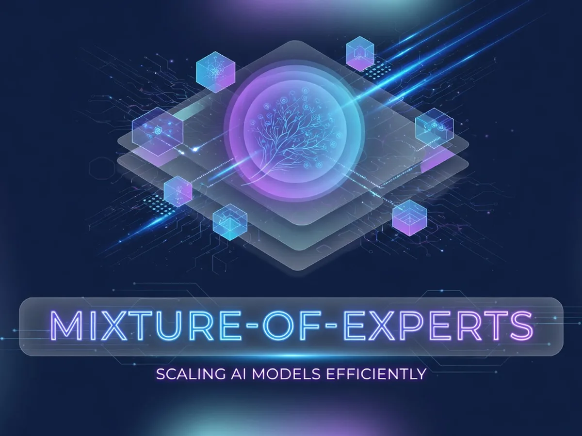
An in-depth look at Mixture-of-Experts (MoE) architecture, its routing mechanisms, training challenges, and production deployment strategies for large-scale AI systems.
As large language models (LLMs) grow beyond hundreds of billions of parameters, dense architectures — where every token activates all weights — become computationally prohibitive. Mixture-of-Experts (MoE) offers a sparse alternative: a model composed of many specialized sub-networks (experts) where only a small subset is active per input. This article explores MoE fundamentals, routing algorithms, training dynamics, and production considerations.
#Why MoE? The Scaling Problem
Dense Transformers scale compute linearly with parameter count. A 1 trillion-parameter dense model requires ~2×10¹² FLOPs per token (forward + backward). At that scale, training time, memory bandwidth, and energy costs dominate. MoE decouples total parameters from active parameters:
- Total parameters can reach trillions (model capacity).
- Active parameters per token stay in the tens of billions (compute budget).
This sparsity enables conditional computation: the model allocates capacity where needed, similar to how the human brain recruits specialized regions for different tasks.
#Core Architecture
An MoE layer replaces a standard feed-forward network (FFN) with E expert FFNs and a router (also called a gate). For each token x:
- Router computes logits g(x) ∈ ℝᴱ (often a linear layer followed by softmax).
- Top-k experts are selected (typically k = 1 or 2).
- Token is dispatched to chosen experts; their outputs are weighted and summed.
          ┌─ Expert 1 ─┐
    x ───►│  Expert 2  │──► y = Σ w_i · Expert_i(x)
          │   ...      │
          └─ Expert E ─┘
               ▲
           Router
Key design choices:
- Expert capacity: maximum tokens an expert can process per batch. Excess tokens are dropped or routed to overflow experts.
- Load balancing: auxiliary loss encouraging uniform expert utilization.
- Expert parallelism: experts distributed across devices (model parallelism).
#Routing Mechanisms
| Router Type | Description | Pros | Cons |
|---|---|---|---|
| Top-k Gating | Softmax + top-k selection | Simple, differentiable | Can cause imbalance |
| Switch Transformer | k=1, no auxiliary loss (uses capacity factor) | Low routing overhead | Requires large capacity factor |
| Expert Choice | Experts select top tokens (reversed) | Perfect load balance | Breaks token-level parallelism |
| Learned Routing | Router trained with RL or differentiable relaxation | Adaptive | Complex, unstable |
Switch Transformer (Fedus et al., 2021) popularized k=1 with a capacity factor (e.g., 1.25× tokens per expert). Dropped tokens are either skipped (inference) or passed through a residual connection (training).
#Training Dynamics & Challenges
#Load Balancing
Without explicit incentives, routers collapse to a few experts. Standard auxiliary loss:
# PyTorch-style pseudo-code
gate_logits = router(x)          # [batch*seq, E]
gate_probs = gate_logits.softmax(-1)
topk_probs, topk_idx = gate_probs.topk(k, dim=-1)

# Load balancing loss
tokens_per_expert = topk_idx.bincount(minlength=E).float()
mean_load = tokens_per_expert.mean()
balance_loss = ((tokens_per_expert - mean_load) ** 2).mean()
Recent work (e.g., DeepSeek-MoE) introduces fine-grained experts (many small experts) + shared experts (always active) to reduce routing variance.
#Communication Overhead
In distributed training (e.g., 3D parallelism: data × tensor × expert), all-to-all communication dispatches tokens to expert devices. This becomes a bottleneck at scale. Optimizations:
- Overlap communication with computation using CUDA streams.
- Hierarchical routing: local experts on same node first, then cross-node.
- Token dropping with dropless variants (e.g., MoE-Layer with fixed assignment).
#Training Stability
MoE models exhibit higher gradient variance. Techniques:
- Expert dropout (randomly disable experts during training).
- Router z-loss: penalize large logits to prevent saturation.
- Gradient clipping per expert.
#Inference & Deployment
#Memory Footprint
Only active experts need GPU memory for weights. With E=64, k=2, active params ≈ 3% of total. However, all experts must reside in memory (or fast storage) for low-latency serving. Solutions:
- Expert offloading: keep cold experts on CPU/NVMe, swap on demand (e.g., FlexGen, DeepSpeed-MoE).
- Quantization: 4-bit experts (GPTQ/AWQ) reduce VRAM by 4× with minimal quality loss.
- Expert merging: combine similar experts post-training (research stage).
#Batching & Scheduling
MoE inference benefits from large batches to amortize all-to-all overhead. Continuous batching (iteration-level scheduling) must group tokens by expert affinity. vLLM and TensorRT-LLM now support MoE with:
- Expert-parallel tensor parallelism (split experts across GPUs).
- Dynamic routing cache for repeated prefixes.
#Decision Matrix: When to Use MoE
| Scenario | Recommendation |
|---|---|
| Model > 100B params, training budget fixed | MoE preferred (2–4× compute savings) |
| Latency-critical, small batch (e.g., chat) | Dense or small MoE (E≤8, k=1) |
| Heterogeneous hardware (CPU+GPU) | MoE with expert offloading |
| Multilingual / multi-domain | MoE excels (experts specialize naturally) |
| Team lacks distributed systems expertise | Start dense; migrate later |
#Real-World Examples
- GLaM (Google, 1.2T params, 64 experts, k=2) — 5× training FLOP reduction vs. GPT-3.
- Mixtral 8×7B (Mistral, 8 experts, k=2) — outperforms Llama-2 70B at 12.9B active params.
- DeepSeek-V2 (236B total, 21B active, 160 experts + 6 shared) — fine-grained design.
- DBRX (Databricks, 132B total, 36B active, 16 experts, k=4) — strong code/math performance.
#Conclusion
Mixture-of-Experts transforms the scaling curve of large models by introducing conditional computation. The architecture shifts complexity from raw FLOPs to routing efficiency, communication topology, and memory hierarchy management. For teams building >100B parameter models, MoE is no longer optional — it’s the default path to cost-effective training and serving. Start with a small expert count (8–16), invest in load-balancing instrumentation, and profile all-to-all latency early. The next frontier: dynamic expert activation (variable k per token) and cross-layer expert sharing to further blur the line between sparse and dense computation.
Related articles
 AI Infrastructure
Alibaba's AI Infrastructure: Architecture, Scale, and Lessons for Engineers
An in‑depth look at Alibaba's AI infrastructure — from custom silicon and high‑performance networking to the Feitian training platform and ModelScope model hub — with practical takeaways for building scalable ML systems.